
Investors and policymakers rely on the investment demand curve to understand how real interest rates influence firms’ capital spending. This article synthesizes core concepts, extensions, and applications to deliver an in-depth, actionable perspective on investment behavior.
What Is the Investment Demand Curve?
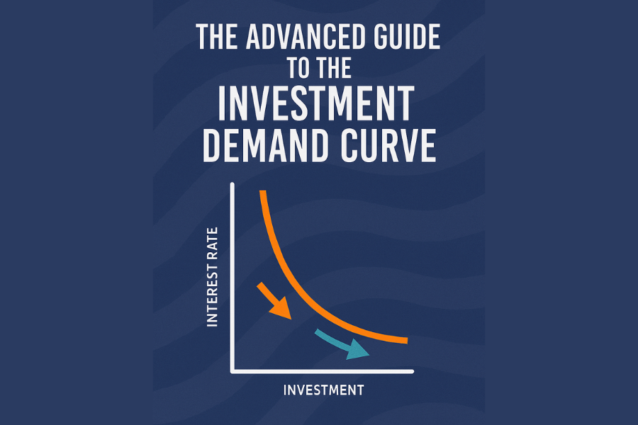
An investment demand curve plots real interest rates against firms’ capital spending. You find rates on the vertical axis. Quantity of investment sits on the horizontal axis. Lower rates unlock more projects that clear firms’ hurdle returns.
According to the Federal Reserve, US nonresidential fixed investment reached $2.23 trillion in 2024 (Federal Reserve 2025).
Why Does the Curve Slope Downward?
Firms list projects by expected real return. Projects with returns above the real interest rate earn approval. Higher rates cut out lower-yield options and shrink investment. Lower rates open the door to more projects and boost investment volume.
What questions do you have when rates fall by 50 basis points? You might ask how many new projects become viable.
How Do Movements Along and Shifts Differ?

Movements along the curve happen when the real rate changes alone. You remain on the same curve but at a new quantity. Shifts occur when nonrate factors change expected returns at every rate.
Examples of shift drivers include
- Tax reforms or investment credits
- Breakthroughs in technology
- Fluctuations in business confidence
What Factors Drive Investment Demand?
Expectations about future sales lift the curve. Favorable tax credits lower firms’ effective cost of funds. High capacity use pushes firms to expand. Tobin’s q above 1 signals market value exceeding replacement cost and spurs spending.
Global R&D outlays reached $2.4 trillion in 2023, up 8 percent over 2022 (OECD 2024).
How Does It Compare to Consumer Demand?
You see two downward slopes, but drivers differ sharply.
| Feature | Investment Demand | Consumer Demand |
| Independent variable | Real interest rate | Product price |
| Dependent variable | Capital spending | Quantity consumed |
| Main motivator | Finance cost and return expectations | Income and preferences |
| Curve shifts triggered by | Tax policy; Tobin’s q; capacity use | Income changes; tastes; substitute prices |
| Elasticity | High sensitivity to rate moves | Varies by product category |
How Does It Fit into Macroeconomic Models?
You link investment demand with consumption to trace the IS curve. A rightward shift in investment moves the IS curve right. Fiscal stimulus might push real rates up and crowd out private investment. Monetary policy guides short-term rates and shapes long-term borrowing costs that you face when funding capital projects.
How Do Researchers Estimate the Curve?
Researchers gather time-series data on real rates and business fixed investment. They add controls for tax changes, capacity utilization, and profitability. Regression or SVAR techniques isolate rate-driven movements. Robust estimates can forecast how a 100 basis-point rate cut might raise investment by 2.5 percent over a year.
What Advanced Theories Extend the Model?
Real Options Theory treats each project as a delayable option and values the choice to wait. DSGE frameworks embed investment demand within full macro models shaped by shocks and expectations. Heterogeneous firms models reflect that some businesses face higher hurdle rates or capital constraints, which flattens the aggregate curve.
What Should You Explore Next?
Have you considered how recent tax overhauls affected capital spending in manufacturing? What happens to investment demand when energy costs surge? How would renewable energy projects reshape the curve if governments offer green subsidies?
By probing these questions, you sharpen your grasp of investment demand as both a predictive tool and a real-world guide to capital allocation.
Final Thoughts
You now see how real rates and nonrate factors shape firms’ capital spending. Tracking shifts in technology, tax policy, and market sentiment adds depth to simple rate-based analysis. Applying advanced models such as real options theory or heterogeneous-firms frameworks brings your forecasts closer to real-world outcomes.
Consider the ripple effects. A rate cut that boosts investment today can lift future productivity, incomes, and overall economic growth. Monitoring investment demand offers early signals on the business cycle, making it a powerful tool for analysts, policymakers, and investors alike.
FAQs
What triggers a movement along the investment demand curve?
A pure change in the real interest rate causes movement along the curve. You remain on the same demand schedule but see a different investment quantity at the new rate.
Which factors shift the investment demand curve?
Tax reforms, investment credits, technological breakthroughs, shifts in business confidence, and changes in expected future demand shift the curve outward or inward.
How do tax incentives affect investment demand?
Tax incentives lower firms’ effective borrowing cost. That action raises project returns and shifts the curve right, increasing investment at every rate.
What role does Tobin’s q play in investment decisions?
Tobin’s q measures the market value of installed capital relative to its replacement cost. A q greater than 1 signals undervalued future returns and prompts firms to invest more.
How do analysts estimate the investment demand curve?
They compile time-series on real rates and fixed investment, control for nonrate drivers, and use regression or SVAR techniques to isolate the rate-investment relationship.
Why use real options theory?
Real options theory values the flexibility to delay or abandon projects. That approach captures strategic decision-making under uncertainty and often explains investment delays during volatile periods.
How does investment demand inform macro policy?
Policymakers use investment responses to rate cuts or fiscal incentives to calibrate IS–LM models, forecast growth, and anticipate crowding-out effects on private spending.
Fuel your curiosity with fast facts and fresh ideas — QuickFast

